Shiny: Performance Tuning with future & promises - The practice
The second part of our blog series on Shiny dealt with the optimization within Shiny applications. We looked at the theoretical part on how Shiny and the packages future & promises work. In the context of these two packages it was presented how they can be used to outsource complex tasks to secondary processes by implementing an asynchronous workflow in order to keep the app accessible for all other users accessing it in parallel. The background for this is provided by the way Shiny works, in which such a task can ensure that not only the current user but also several users at the same time have to wait for the task to be completed. Some examples of these tasks, which we call “process-blocking” tasks, will be implemented in this article by an example app with future & promises. Here, the transfer from theory to practice will be shown. At first, an overview of the final app and its functionality will be given. Afterwards, selected code examples are used to show how the processes can be programmed in the context of the future & promises syntax.
Would you like to try out the procedures explained here directly with the app? Here you can find the code!
The goal - explanation of the test application and Web UI
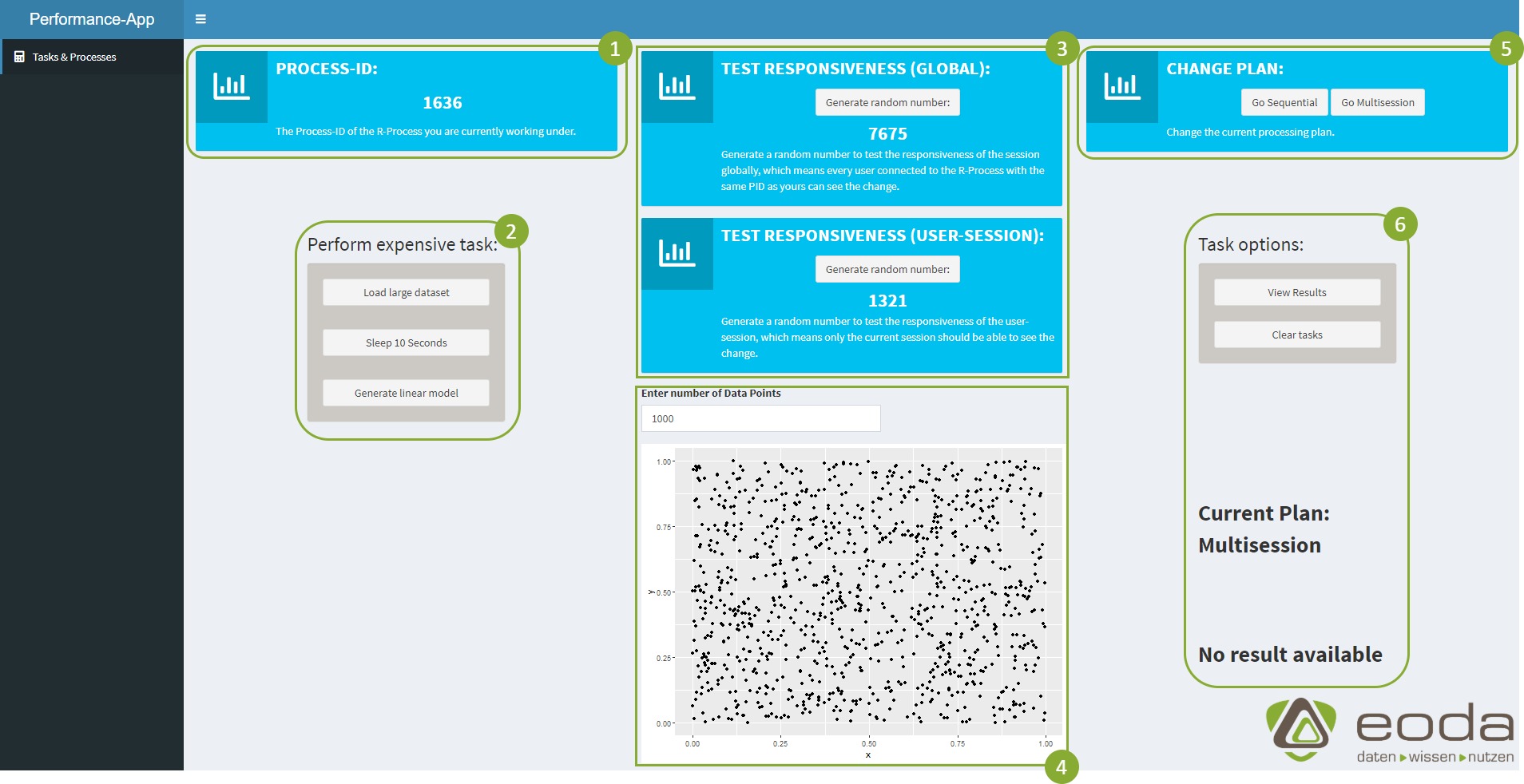
- Info-PID: The current process ID of the R-process to which the user is connected can be read here.
- Start task: For testing the implementation, complex and process–blocking tasks can be started here. These include:
- Loading a CSV file with 1.500.000 lines.
- Shutting down the process for 10 seconds.
- The calculation of a linear regression model based on two vectors with 5,000,000 entries each.
- Availability test: It can be tested whether the current process is responsive or blocked by the execution of a task. The availability of the global R process running the Shiny app is distinguished from the individual user session (the distinction will be interesting for testing later).
- “Live” task: A task by entering the number of data points can be started here. It will display the result “live” in the plot below. In connection with point 2 this is only used to present different possibilities for implementing the asynchronous workflow.
- Change plan: Here you can change the current plan from a sequential to an asynchronous (multisession) workflow. In this way, an evaluation of the behavior of the app regarding both possibilities are possible.
- Information/results: The tasks started from point 2 can be viewed and reset. In addition, information about the current plan and the status of the tasks can be found here.

The components - How is the asynchronous workflow implemented?
1library(shiny)
2library(future)
3library(promises)
4library(dplyr)
⋮
10plan(multisession)
11
12reac <- reactiveValues(
13plan = "Multisession",
14random_number = round(runif(1, min = 1000, max = 9999))
15)
⋮
Code block #1
In order to understand the functionality of the app and the associated use of future & promises, the structure of the app is now described by using code snippets.
At the beginning the necessary packages are added. In this example multisession the initial plan for the app is set in line 10. This means that the code blocks implemented with future & promises are executed asynchronously by default. In lines 12-15, two reactive variables are initialized, which contain the current plan and one of the random numbers for the availability test. Since the definition here is done in the global.R (i.e. outside the server), the variables are valid for all users connected to the R process.
In contrast, additional reactive variables are defined in the server, which are therefore session-specific, i.e. they are created individually for each user at the start of a session.
Code block #2
The session-specific variables contain the second random number for the availability test as well as information and results of the current/completed tasks.
Based on the necessary definitions, you can now start with the first task of the implementation: loading the CSV file.
1function(input, output, session)}
2
3reac_sess <- reactiveValues(
4random_number = round(runif(1, min = 1000, max = 9999)),
5active_task = FALSE,
6current_task = "task_null",
7dataset = NULL,
8model = NULL
9)
⋮
Code block #3
In lines 65 & 66 a progress bar is created and started. It also shows the user the status of the task.
Attention: Since the tasks are executed in a separate R process, the function withProgress provided by Shiny cannot be used.
In lines 68 – 71 the import of the CSV file is started as an asynchronous process. With future({ Code block }) the execution of the code is swapped to another R process, according to the plan we selected at the beginning. The console output on line 70 is used to trace the code, i.e. which process ID executed the code. Lines 72 – 77 define what happens once the execution is complete. In this case, the pipe operator %…>% from the promises packet in line 71 is important. It ensures that the subsequent code block is not executed until the asynchronous task has successfully completed.
Finally deletes the progress bar, regardless of whether the commands were successful before. Clearing the progress bar is necessary if the previous asynchronous block could not be completed successfully. Therefore, this block is also added to the end of the code chain with the usual %>% pipe.
⋮
63observeEvent(input$task_loaddata, {
64
65p <- Progress$new()
66p$set(value = 0.5, message = "Load Dataset")</span
67
68future({
69cat(paste0("--- Executed task 'Loading dataset' under PID: ", Sys.getpid(), "\n"))
70read.csv("1500000 Sales Records.csv")
71}) %...>%
72{
73reac_sess$dataset <- .
74reac_sess$current_task <- "task_load"
75reac_sess&active_task <- TRUE
76cat(paste0("--- Finished task 'Loading dataset' under PID: ", Sys.getpid(), "\n"))
77} %>%
78finally(~p$close())
79})
⋮
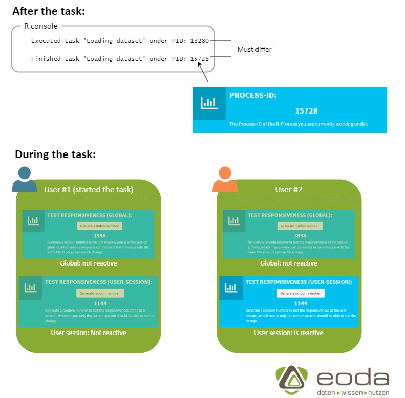
After implementing the first asynchronous task, it can be tested directly. This should result in the following behavior of the app:

Code block #4
Lines 81 – 102 contain the implementation to shut down the process for ten seconds. At first, this implementation runs identically to the loading of the data record. The adjustment of the progress bar in line 89, after five seconds of standstill, should be emphasized. It is often necessary to have an overview of the task in the main process even while the asynchronously started task is being executed. It should also be possible to make changes, such as adjusting the progress bar. These changes must usually be made outside the future environment, because without additional packages such as ipc, communication between the various processes is not possible.
⋮
81observeEvent(input$task_sleep, {
82
83p <- Progress$new()
84p$set(value = 0.1, message = "Begin Sleeping")
85
86future({
87Sys.sleep(5)
88}) %...>%
89{ p$set(value = 0.6, message = "Slept for 5 seconds") } %...>%
90{
91future({
92Sys.sleep(5)
93cat(paste0("--- Executed task 'Sleeping' under PID: ", Sys.getpid(), "\n"))
94})
95} %...>%
96{
97reac_sess$current_task <- "task_sleep"
98reac_sess$active_task <- TRUE
99cat(paste0("--- Finished task 'Sleeping' under PID: ", Sys.getpid(), "\n\n"))
100} %>%
101finally(~p$close())
102})
⋮
Code block #5
In lines 11 – 19 and 173 – 180 the live task is implemented. This shows another method of using the asynchronous workflow. In lines 11 – 19, the dataset for the graphic is stored as a reactive variable, in which the creation of the data set starts as an asynchronous process. In lines 173 – 180 the data set can finally be retrieved and drawn. It is important that the reactive variable plot_df does not contain the dataset. However, the future object has to contain it, since it is responsible for the creation of the dataset. Therefore, the drawing process must be added to the dataset with a promise-pipe (%…>%). While the dataset is created and drawn “live”, the same behaviour should occur as when the CSV file is loaded asynchronously.
The asynchronous workflow can be implemented in many other ways, for example, the future block from the last code block could be implemented directly in the renderPlot({ … }) environment. Furthermore, the results of the future blocks can be managed in many different ways (e.g. error handling for failed tasks/explicit function statements for successful tasks with then( … )).
⋮
11plot_df <- eventReactive(input$number_cap, {
12cap <- input$number_cap
13
14future({
15x <- runif(cap)
16y <- runif(cap)
17data.frame("x" = x, "y" = y)
18})
19})
⋮
173output$number_plot <- renderPlot({
174plotdf() %...>%
175{
176df <- .
177ggplot(df, aes(x = x, y = y)) +
178geom_point()
179}
180})
⋮
Conclusion
Even if the implementation of tasks with future & promises only serves one specific aspect of optimizing Shiny applications, this can contribute significantly to the increase of user experience (UX) satisfaction. The optimization points shown above show their strengths when many users work on the app at the same time. If the individual processes such as database accesses, rendering of graphics, optimization of the importing of data for their runtime are required, then a complete package can be put together in cooperation with the asynchronous workflow and the horizontal storage capability. This combines the extensive possibilities of Shiny applications with the modern demands on performance and user-friendliness.
Do you have problems with the performance of your Shiny apps? We are happy to help you with the conception of your applications, from the initial design to the performance optimization of existing infrastructures and apps. Contact us!